Appendix¶

Bias Variance Tradeoff¶

In statistical learning, we learn the mapping from \(X\) to \(Y\), where \(X\) is a matrix of size \(N \times p\). \(N\) denoting the number of data points we have observed, and each data point is a vector in \(p\) dimensions. \(Y\) is the value of the response for the observed data points and is of shape \(N \times 1\). We wish to learn the mapping \(f:\mathbb{R}^{p} \rightarrow \mathbb{R}\) so that we can predict the value of \(Y\) for obserations where true \(Y\) is not known. \((X, Y)\) is the training data avaiable to us to learn the function \(f\). Additionally, there is some noise component also present in the observed \(Y\)

\[ \begin{aligned} Y = f(X) + \epsilon\end{aligned} \]

which is immeasureable, independent of \(X\) and other noise values, and has \(0\) mean, \(E[\epsilon] = 0\). We obtain a best guess \(\hat{f}\) and make predictions as

\[ \begin{aligned} \hat{Y} = \hat{f}(X)\end{aligned} \]

where \(\hat{Y}\) is our best estimate of \(Y\). We use least squares error to measure how good or bad our estimate \(\hat{f}\) is

\[ \begin{aligned} E[(Y - \hat{Y})^{2}] &= E[(f(X) + \epsilon - \hat{f}(X))^{2}] = E[(f(X) - \hat{f}(X))^{2} + \epsilon^{2} + 2\epsilon f(X) - 2\epsilon \hat{f}(X)]\newline &= E[(f(X) - \hat{f}(X))^{2}] + Var(\epsilon)\newline Var(\epsilon) &= E[\epsilon^{2}] - E[\epsilon]^{2} = E[\epsilon^{2}]\end{aligned} \]

\(Var(\epsilon)\) is the irreducible error since it will always be present. A good model will bring the reducible error \(E[(f(X) - \hat{f}(X))^{2}]\) as close to zero as possible.

Let \(x_{0}\) denote a \(d\) dimensional data point. The bias variance tradeoff is derived by taking expectation across \(D\) datasets

\[ \begin{aligned} E_{D}[(y_{0} - \hat{y}\_{0})^{2}] &= E_{D}[(f(x_{0}) + \epsilon - \hat{f}(x_{0}))^{2}]\newline &= E_{D}[(f(x_{0}) + \epsilon - \hat{f}(x_{0}) + E_{D}[\hat{f}(x_{0})] - E_{D}[\hat{f}(x_{0})])^{2}]\newline &= E_{D}[(\epsilon + (f(x_{0}) - E_{D}[\hat{f}(x_{0})]) + (\hat{f}(x_{0}) - E_{D}[\hat{f}(x_{0})]))^{2}]\newline &= E_{D}[\epsilon^{2}] + E_{D}[(f(x_{0}) - E_{D}[\hat{f}(x_{0})])^{2}] + E_{D}[(\hat{f}(x_{0}) - E_{D}[\hat{f}(x_{0})])]\newline &+ 2E_{D}[\epsilon(f(x_{0}) - E_{D}[\hat{f}(x_{0})])] + 2E_{D}[\epsilon (\hat{f}(x_{0}) - E_{D}[\hat{f}(x_{0})])] \newline &+ 2E_{D}[(f(x_{0}) - E_{D}[\hat{f}(x_{0})]) + (\hat{f}(x_{0}) - E_{D}[\hat{f}(x_{0})])]\newline &= Var(\epsilon) + (f(x_{0}) - E_{D}[\hat{f}(x_{0})])^{2} + Var(\hat{f}(x_{0})) + 0 + 0\newline &- 2E_{D}[(f(x_{0}) - E_{D}[\hat{f}(x_{0})](E_{D}[\hat{f}(x_{0}] - E_{D}[\hat{f}(x_{0})])\newline E_{D}[(y_{0} - \hat{y}\_{0})^{2}] &= Var(\epsilon) + Bias(\hat{f}(x_{0}))^{2} + Var(\hat{f}(x_{0})) \end{aligned} \]

where we have used the following facts

\(\epsilon\) is independent of both \(f\) and \(\hat{f}\)\(E_{D}[\epsilon \times f \;or\; \hat{f}] = E_{D}[\epsilon] * constant = 0\)
\(E[f(x_{0})] = f(x_{0})\) since \(f\) is the true function and fixed/constant
\(E_{D}[\hat{f}(x_{0})] = constant\) and represents \(\hat{f}\) averaged across all the datasets

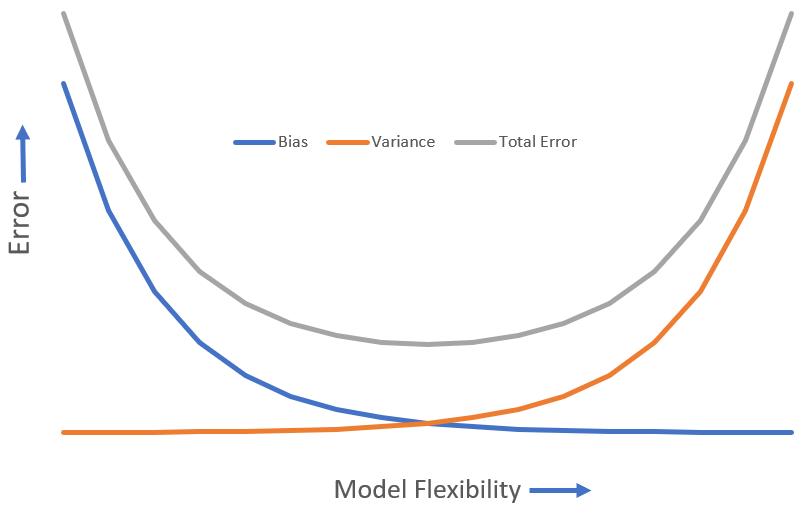
The last equation consists of all positive terms and is called the bias variance tradeoff. \(Var(\epsilon)\) is the irreducible error. Variance of \(\hat{f}\) is calculated across all the datasets. The bias term represents how off our estimate is from the true value. As model flexibility increases, we get a reduction in the bias, but the variance increases, and vice versa.