Latent Dirichlet Allocation (LDA)

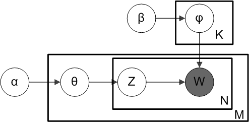
LDA is a method used in topic modelling where we consider documents as mixture models. Suppose we have $M$ documents in our corpus (collection of documents) and the $i^{th}$ document consists of $N_{i}$ words (total words in vocabulary is $V$). We introduce a latent variable which denotes topics, and assume a total of $K$ topics. Each document is assumed to be a distribution/mixture over topics, and each topic a mixture/distribution over words.

In our definition, document is a distribution over topics. Hence, $\sum p(topic \vert document) = 1$. Thus, we can define this probability vector as $\boldsymbol{\theta}$ which can be sampled from a dirichlet distribution $Dir(\boldsymbol{\alpha})$ (to impose the constraint that all probabilities in a given row sum to 1). Similarly, $\sum p(word \vert topic) = 1$. We define this vector as $\phi$ sampled from $Dir(\boldsymbol{\beta})$ where both $\boldsymbol{\alpha}$ and $\boldsymbol{\beta}$ are typically sparse.

Then the generative model for the corpus becomes

1. Generate the matrix $\boldsymbol{\Theta}$ of shape $M \times K$ where each row $\boldsymbol{\theta}_{m} \sim Dir(\boldsymbol{\alpha})$ is a distribution over topics for document $m$.

2. Generate the matrix $\boldsymbol{\phi}$ of shape $K \times V$ where each row $\boldsymbol{\phi}_{k} \sim Dir(\boldsymbol{\beta})$ is a distribution over words for topic $k$.

3. After fixing the values in the distributions, for each document $i$ in the corpus and each word at position $j$ in the document

   1. Select a topic $z_{i,j}$ from $\boldsymbol{\theta}_{m}$ using discrete inverse transform method (refer to sampling section in probability notes) or simply sampling discrete random variable from a discrete probability distribution.

   2. Select a word $w_{i,j}$ from $\boldsymbol{\phi}_{z_{i,j}}$ using the same sampling procedure as above.

Our random variables then are $\boldsymbol{\Theta}, \boldsymbol{\Phi}, \boldsymbol{Z}$ and $\boldsymbol{W}$, with the data $\boldsymbol{W}$ known. The total likelihood of the model becomes \begin{gather} P(\boldsymbol{W},\boldsymbol{Z},\boldsymbol{\Theta}, \boldsymbol{\Phi}) = \prod_{i=1}^{M} p(\boldsymbol{\theta}_{i}) \bigg( \prod_{j=1}^{N_{i}} p(z_{i,j} \vert \boldsymbol{\theta}_{i}) p(w_{i,j} \vert z_{i,j}) \bigg)\newline \text{with} \quad \boldsymbol{\theta}_{i} \sim Dir(\boldsymbol{\alpha}), \; p(z_{i,j} \vert \boldsymbol{\theta}_{i}) = \boldsymbol{\Theta}_{i,z_{i,j}}, \; p(w_{i,j} \vert z_{i,j}) = \boldsymbol{\Phi}_{z_{i,j},w_{i,j}}\newline LL(\boldsymbol{W},\boldsymbol{Z},\boldsymbol{\Theta}, \boldsymbol{\Phi}) = \sum_{i=1}^{M} log(p(\boldsymbol{\theta}_{i})) + \bigg( \sum_{j=1}^{N_{i}} log(p(z_{i,j} \vert \boldsymbol{\theta}_{i})) + log(p(w_{i,j} \vert z_{i,j})) \bigg)\newline \end{gather}