Hierarchical Clustering

$K$-means suffers from the disadvantage that the number of clusters needs to be specified beforehand. Hierarchical does not require such a consideration beforehand. here we dicsuss the bottom-up or agglomerative clustering approach. Hierarchical clustering is visualized using a dendogram which is a tree like diagram draw upside down. Starting from the bottom, branches are originate from the individual data points and slowly start merging as we move upward. The earlier the branches merge, the similar the data points are and vice versa. (Be careful to not judge the similarity from the proximity on the horizontal axis)

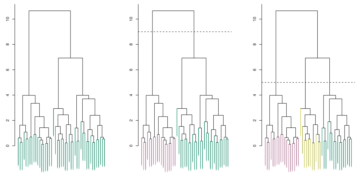
The number of clusters is simply determined by the height at which we made the cut. The middle figure in figure above shows a cut at height 9 which results in two branches and thus two clusters.

Changing the height from the highest value to the lowest value will result in 1 and $n$ clusters respectively. Thus, we do not need to specify the number of clusters beforehand but it is rather to be chosen by us based on the height. This height can be seen similar to $K$ in $K$-means clustering.

The inherent nesting of the clusters as indicated visually by the dendogram may not be possible in every data set and there will be cases when $K$-means clustering may be superior.

Algorithm

Hierarchical Clustering is performed in a bottom-up approach. Start with $n$ clusters where each observation is it’s own cluster. Define a dissimilarity measure between each pair of observation. This can be Euclidean distance as well. Now, cluster the observations that are least dissimilar into the same group, which will give us $n-1$ clusters. Again use the dissimilarity measure to group two similar observations until the total number of clusters is 1.

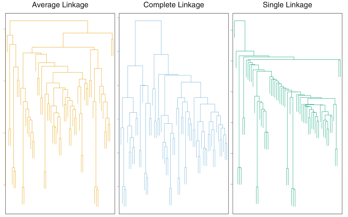
Consequently, there will be cases when we need to determine the dissimilarity between a group and an observation or a pair of groups. This is done using linkage. Four types of linkages used are complete, average, single and centroid. Average and complete linkages are preferred over single linkages, and all three are more popular than centroid linkage. Average and complete likages will usually give balanced dendograms.

Following are teh descriptions of individual types of linkages

• Complete Maximal intercluster dissimilarity. Take the maximum of the pairwise dissimilarity between observations of cluster A and cluster B.

• Single Minimum intercluster dissimilarity. Take the minimum of the pairwise dissimilarity between observations of cluster A and cluster B.

  Single linkage can result in extended trailing clusters in which single observations fuse one at a time.

• Average Mean intercluster dissimilarity. Take the average of the pairwise dissimilarity between observations of cluster A and B.

• Centroid Take the dissimilarity between the centroid of cluster A and B. Centroid linkages can result in undesirable inversions.

The algorithm can be summarized as follows

1. Start with $n$ clusters where each observation is it’s own cluster. Compute $n(n-1)/2$ pairwise dissimilarity measures between all pairs.

2. For $i=n, n-1, \ldots, 2$

   1. Compute the pairwise dissimilarity between all $i$ clusters and take the two clusters with the least dissimilarity (or highest similarity). Fuse them into a single cluster. The dissimilarity measure is also indicative of the height in the dendogram where the two clusters fuse.

   2. Recompute the pairwise dissimilarity between the $n-1$ clusters.

The above is the case of agglomerative clustering which is a bottom up appraoch. Top down approaches are called divisive clustering, since they will recursively split observations into two clusters such that the inter cluster dissimilarity is the highest.