Shrinkage Methods and Regularization

Instead of using a subset of predictors, we can also use all of the predictors and shrink the coefficients towards zero. This approach significantly reduces the variance in the model estimates as the subset selection methods often suffer from high variance. The famous ones here are Ridge Regression and Lasso Regression.

Ridge Regression

Ridge Regression is very similar to the least square estimate for linear regression except that we add a term corresponding to the squared sum of the regression coefficients in the error. \begin{align} error &= RSS + \lambda \sum_{j=1}{p}\beta_{j}^{2}\newline &= (Y-X\beta)^{T}(Y-X\beta) + \lambda \beta^{T}\beta \end{align} $\lambda$ is a tuning parameter that needs to be chosen separately. It acts as a weight between the error in the data and how large are the regression coefficients. It is also known as the shrinkage penalty.

Note that we will not include the intercept term in shrinkage because it is simply the mean estimate of the model when all the predictors are zero and may not necessarily zero. Thus the above model includes $p$ terms in $\beta$. When the model inputs are all centered (which is always preferred), the intercept can be calculated in the end as simply $\sum_{i=1}^{n}y_{i}/n$

Using least squares estimate, \begin{align} error &= (Y-X\beta)^{T}(Y-X\beta) + \lambda \beta^{T}\beta\newline \frac{\partial error}{\partial \beta} &= 0\newline \implies 0 &= -Y^{T}X - Y^{T}X + \beta^{T}X^{T}X + \beta^{T}X^{T}X + \lambda \beta^{T} + \lambda \beta^{T}\newline \beta^{T}(X^{T}X + \lambda I) &= Y^{T}X\newline (X^{T}X + \lambda I)^{T}\beta &= X^{T}Y\newline (X^{T}X + \lambda I)\beta &= X^{T}Y\newline \beta &= (X^{T}X + \lambda I)^{-1}X^{T}Y \end{align} $\lambda = 0$ will result in the simple least squares regression while $\lambda \to \inf$ will force the coefficients to go towards zero.

As is clear from the formula, the error term is sensitive to the actual scale of the coefficients which is ultimately dependent on the predictors themselves. In a simple least squares regression, the coefficients will scale up and down depending on how the data is scaled. The same is not true for Ridge Regression.

Hence when using Ridge Regression, it is always advisable to standardize the predictors before training the model using \begin{align} \tilde{x}_{ij} = \frac{x_{ij} - \bar{x_{j}}}{\sqrt{\frac{1}{n}\sum_{i=1}{n}(x_{ij}-\bar{x}_{j})^{2}}} \end{align}

The success of Ridge Regression is based in the bias variance tradeoff. If the data is linear, simple linear regression will have a very low bias but high variance, making it sensitive to the training data. As $\lambda$ is introduced, it forces the model to have less flexibility by reducing the coefficiets value and subsequently their power on the prediction. This causes a reduction in the variance at expense of slight increase in bias. However, this trend is not monotonic with increasing $\lambda$ and the appropriate value must be chosen based on the errors observed.

Ridge regression will tend to give similar coefficient values for correlated variables.

Lasso Regression

Notice that Ridge Regression will try to reduce the value of some of the coefficients, but it will never set them to exactly zero. Hence, we will end up using all the $p$ predictors in the model which may not be interpretable if the value of $p$ is large.

Lasso Regression comes over this disadvantage by defining the error as \begin{align} error &= RSS + \lambda \sum_{j=1}^{p}\mid \lambda_{j} \mid \end{align}

which does not include the intercept. When $\lambda$ is sufficiently large, Lasso Regression forces some of the variables to be exactly zero. This is very useful in reducing the subset of variables that we use in the model, thereby increasing model interpretability.

Lasso Regression can give different coefficient values to correlated variables.

Similar to Ridge Regression, if we have standardized the input variables, the intercept is simply the average of the $y$’s and can be computed in the end after obtaining the other coefficients.

Alternative Formulation to Ridge and Lasso Regression

These regressions can also be considered as solving a constrained optimisation problem \begin{alignat}{2} &\minimize_{\beta} \left\{\sum_{i=1}^{n} (y_{i} - \beta_{0} - \sum_{j=1}^{p}\beta_{j}x_{ij})^{2} \right\} \quad \text{subject to} &&\sum_{j=1}^{p}\beta_{j}^{2} \leq s \newline &\minimize_{\beta} \left\{\sum_{i=1}^{n} (y_{i} - \beta_{0} - \sum_{j=1}^{p}\beta_{j}x_{ij})^{2} \right\} \quad \text{subject to} &&\sum_{j=1}^{p}\mid \beta_{j} \mid \leq s \end{alignat} for Ridge and Lasso regression respectively. This holds true because these regressions are effectively trying to limit the size of the coefficients themselves. For $\lambda = 0$, we have no bound on the size and $s$ in equations above is close to $\inf$. As $\lambda$ increases, $s$ will start to decrease and be $0$ for $\lambda \to \inf$.

The equations above can be interpreted as finding the minimum RSS among the points that lie inside the geometric shapes defined by the constraints. For $p = 2$, Ridge defines a circle $\beta_{1}^{2} + \beta_{2}^{2} \leq s$ and Lasso defines a diamond $\mid \beta_{1} \mid + \mid \beta_{2} \mid \leq s$.

Variable Selection Property of Lasso Regression

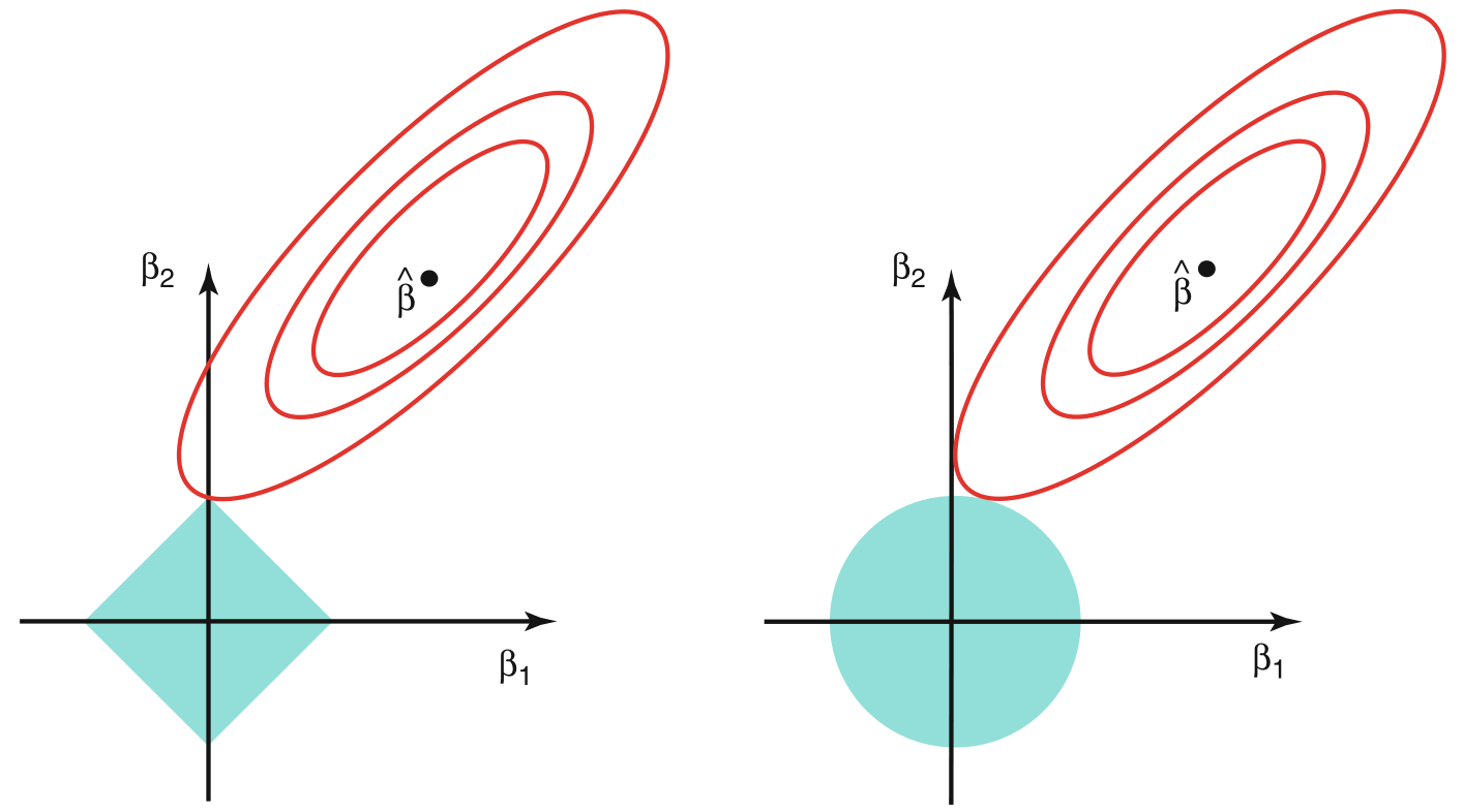
In the figure above, $\hat{\beta}$ corresponds to the least squares estimate of $\beta$ and the contours in red colour show the same value of RSS. The blue coloured regions correspond to the constraints defined above (diamond for lasso and circle for ridge).

Clearly, circle being a smooth shape, the lowest RSS contour will not usually touch it at one of the axis points. However, for the sharp diamond shape, the least RSS value is likely to be encountered along the axis. The shapes of the constraint regions can be controlled through $\lambda$ and for lasso, more constrained models (small $s$ or higher $\lambda$) will cause more of the coefficients to be zero. The argmuents are very well valid in higher dimensions as well.

Bayesian Interpretation

Lasso and Ridge Regression are also natural solutions when the the coefficients are assumed to have certain specific priors.

\begin{align} p(\beta|X,Y) &\propto f(Y|X,\beta)p(\beta|X) = f(Y|X,\beta)p(\beta) \quad \text{assuming X is constant}\newline Y &= \beta_{0} + \beta_{1}X_{1} + \cdots + \beta_{p}X_{p} + \epsilon\newline \text{Assume, } p(\beta) &= \prod_{j=1}^{p} \beta_{p} \quad \text{for some density function $g$} \end{align}

The following are observed for different priors on $\beta$

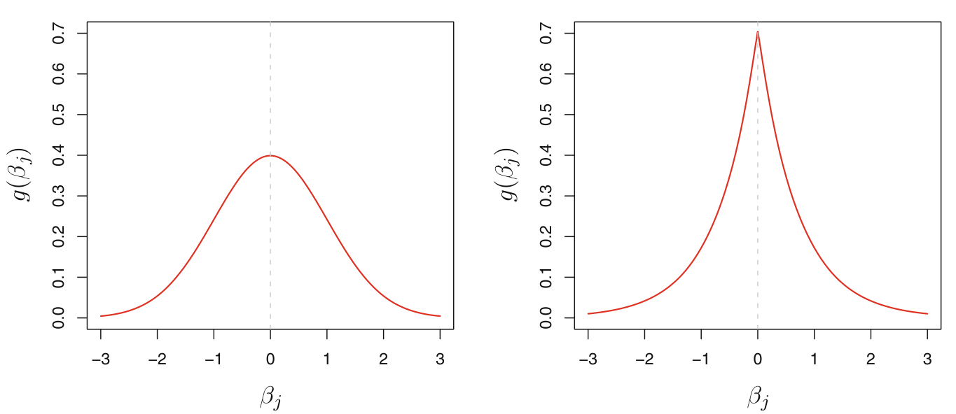
• When the density function of $\beta_{j}$ is assumed to be a standard normal, the posterior is same as solving the ridge regression error function

• When the density function is assumed to be a double exponential, the posterior is the same as solving lasso error function

From the visuals of the priors in the earlier figure, double exponential is steeply peaked at zero, which clearly implies that the prior itself assumes some of the coefficients are likely zero. On the other hand, the gaussian priod is flatter and does not necessarily require the coefficients to be zero.

Elastic Net

Both Lasso and Ridge regression offer their own set of advantages. Ridge helps shrink down coefficients and variance, while lasso helps in variable selection. Elastic Net aims to combine both of these together to do both shrinkage and variable selection. The loss function for Elastic Net is \begin{align} error &= (Y-X\beta)^{T}(Y-X\beta) + \lambda(\alpha\beta^{T}\beta + (1-\alpha)\sum_{j=1}^{p}\mid \beta_{j} \mid)\newline \text{or,} \quad &= RSS + \lambda\sum_{i=1}^{p} (\alpha \beta_{j}^{2} + (1-\alpha)\mid \beta_{j} \mid) \end{align}

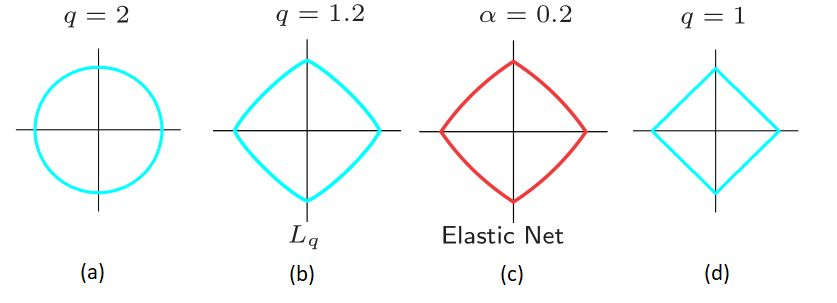
Based on the Bayesian interpretation, one can expect that Elastic Net has the priors distributed in the form $\mid \beta \mid ^{q}, q \in (1,2)$. However, this formulation gives us rounded edges along the axis (as opposed to corners in case of lasso or $q=1$). Elastic Net slightly modifies this to have similar shape to $\mid \beta \mid ^{q}, q \in (1,2)$ but with sharp corners which allows enforcing some coefficients to zero.