Generalized Additive Models

The approches discussed above are extensions of the linear regression model for a single predictor by introducing more flexbility into the models. This idea can be extended for $p$ predictors in the framework of Generalized Additive Models. These are applicable for both classification and regression.

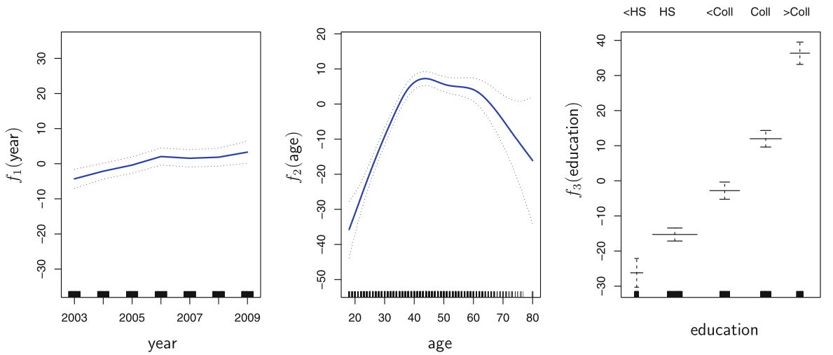
\begin{align} \hat{y}_{i} &= \beta_{0} + \sum_{j=1}^{p} \beta_{j} x_{ij} \quad \text{Linear Rgerssion}\newline \hat{y}_{i} &= \beta_{0} + \sum_{j=1}^{p} f_{j}(x_{ij}) \quad \text{Generalized Additive Models} \end{align} where $f_{i}(x)$ are non-linear smooth functions applied to each of the predictors separately.

Each of the functions above can be fit using all of the sections defined above. For example, some of the predictors can be smooth splines, some can be just dummy variables, and some can be polynomials. Thus, we expand from $p$ predictors to a multitude of them, where we can choose a different expansion method for each of them individually. We have combined individual simple linear regression models into a general framework for $p$ predictors.

Separate non-linear functions for three different variables. y-axis is the response. Left two plots are amoothing splines with different degrees of freedom. Right plot is dummy variables (one hot encoded).

Fitting smoothing splines is not trivial as the loss function is not simple least squares. However, softwares can still fit using partial residuals. We repeatedly update the fit for a single predictor, keeping the others constant.

Summarizing,

GAMs allow us to fit a non-linear $f_{j}$ to each $X_{j}$, so that we can automatically model non-linear relationships that standard linear regression will miss. This means that we do not need to manually try out many different transformations on each variable individually.
The non-linear fits can potentially make more accurate predictions for the response $Y$ .
Because the model is additive, we can still examine the effect of each $X_{j}$ on $Y$ individually while holding all of the other variables fixed. Hence if we are interested in inference, GAMs provide a useful representation.
The smoothness of the function fj for the variable Xj can be summarized via degrees of freedom.
The main limitation of GAMs is that the model is restricted to be additive. With many variables, important interactions can be missed. However, as with linear regression, we can manually add interaction terms to the GAM model by including additional predictors of the form $X_{j} \times X_{k}$. In addition we can add low-dimensional interaction functions of the form $f_{jk}(X_{j}, X_{k})$ into the model; such terms can be fit using two-dimensional smoothers such as local regression, or two-dimensional splines.