t-Distribution¶

Let $Z$ be a standard normal random variable and let $\chi_{n}^{2}$ be a chi-square random variable. Assuming these two random variables are independent, the random variable $T_{n}$ is

\[ \begin{aligned} T_{n} = \frac{Z}{\sqrt{\chi_{n}^{2}/n}} \end{aligned} \]

is said to have a t-distribution with $n$ degrees of freedom.

This distribution is symmetric around the normal, and as $n$ increases, the distribution becomes more and more like the standard normal distribution.

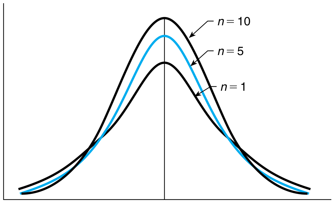
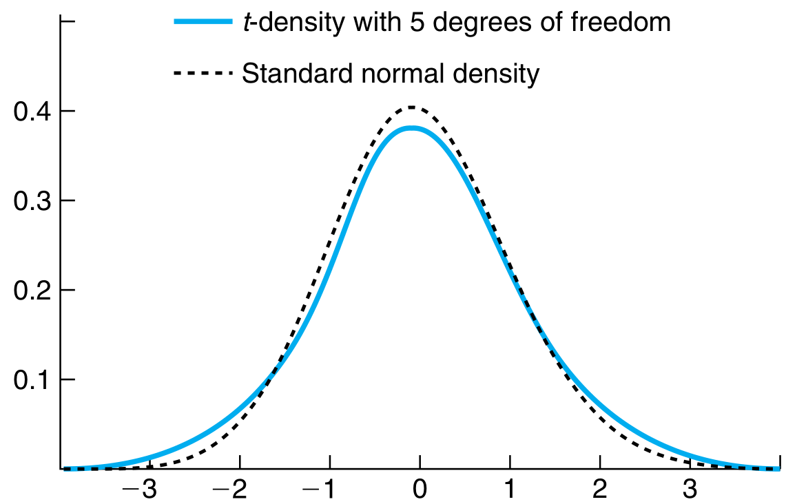
t-distribution for different degrees of freedom

From the above figure , we see that t-distribution is heavier tailed than a standard normal. Translation, this means that a larger value is more likely to occur under a t-distribution than a standard normal. Furthermore, the heavy tails imply more variance than the standard normal.

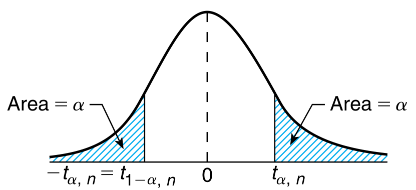
For $\alpha$ between $0$ and $1$, let $t_{\alpha, n}$ be such that

\[ \begin{aligned} P(T_{n} \geq t_{\alpha, n}) = \alpha \end{aligned} \]

By symmetry around the origin,

\[ \begin{aligned} P(T_{n} \leq -t_{\alpha, n}) &= \alpha\newline \text{or} \quad P(T_{n} \geq -t_{\alpha, n}) &= 1 - \alpha\newline \text{and,} \quad -t_{\alpha, n} &= t_{1 - \alpha, n} \end{aligned} \]

These standard values are available in math charts since they form the basis of the t test.

Mean and Variance¶

The following are stated without proof

\[ \begin{aligned} E[T_{n}] &= 0\newline Var(T_{n}) &= \frac{n}{n-2}\newline \end{aligned} \]

In the limit of large $n$, the variance is close to $1$, which is consistent with the fact that the distribution resembles a standard normal in that limit.