Interval Estimates

The MLE estimates calculated above are estimates and do not reflect the true value. We expect the true value of the parameter to be close to the estimate, but not exactly equal to it. Hence, it makes sense to give an interval instead of a single estimate to reflect our confidence in the estimated value of the parameter.

Suppose the parameter is denoted by $\theta$ and lies in a set $\Omega$. For some $0 < \alpha < 1$, and statistics $L$ and $U$ of the sample of random variables, the $(1-\alpha)100%$ confidence interval is $(L,U)$ if \begin{align} 1-\alpha = P_{\theta}(\theta \in (L, U)) \end{align}

implying that if the experiment is repeated several times (draw the sample and calculate the interval), $(1 - \alpha)100%$ times, the constructed interval will contain the true value of the parameter $\theta$.

NOTE: The calculations of intervals do not imply that $\theta$ is contained in the interval with $(1-\alpha)100%$ confidence. We calculate an interval that falls on $\theta$ or traps $\theta$ rather than telling the interval that $\theta$ falls in.

Usually, to obtain the interval, we will first find a pivot (or central) point of our interval using an existing statistic (say MLE) and then construct an interval using statistical properties of the estimate/random variables.

Efficiency of the Interval Estimate

For two estimates of the interval $L_{1}, U_{1}$ and $L_{2}, U_{2}$, we say that the former is more efficient if its a narrower interval, i.e., \begin{align} E_{\theta}\squarebr{U_{1} - L_{1}} < E_{\theta}\squarebr{U_{2} - L_{2}} \quad \forall \theta \in \Omega \end{align}

Confidence interval for Mean of Normal Distribution when Variance is Known

Consider the problem of estimation of the mean of a normal distribution with known variance $\sigma^{2}$. Since we know that the MLE for mean is just the sample mean, and the sample mean follows a normal distribution, \begin{align} P(-1.96 < \frac{\overline{X} - \mu}{\sigma / \sqrt{n}} < 1.96) &= 0.95 \quad\text{using standard normal tables}\newline \text{or,}\quad P(\overline{X} - 1.96\frac{\sigma}{\sqrt{n}}< \mu < \overline{X} + 1.96\frac{\sigma}{\sqrt{n}}) &= 0.95 \end{align} Thus, we are 95% confident that the true value of the mean lies in the range \begin{align} (\overline{X} - 1.96\frac{\sigma}{\sqrt{n}}, \overline{X} + 1.96\frac{\sigma}{\sqrt{n}}) \end{align}

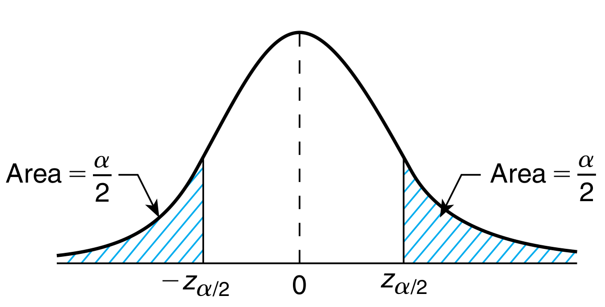
This trick to calculate the confidence interval can be generalized for any value of confidence. Recall that \begin{align} P(Z > z_{\alpha}) = \alpha\newline P(Z < -z_{\alpha}) = \alpha \end{align}

Hence, for a given confidence level $\alpha$, the two sided confidence interval is \begin{align} P(-z_{\alpha /2} < Z < z_{\alpha /2}) &= 1 - \alpha\newline P(-z_{\alpha /2} < \sqrt{n}\frac{\overline{X} - \mu}{\sigma} < z_{\alpha /2}) &= 1 - \alpha\newline P(\overline{x}-z_{\alpha /2}\frac{\sigma}{\sqrt{n}} < \mu < \overline{x}-z_{\alpha /2}\frac{\sigma}{\sqrt{n}}) &= 1 - \alpha\newline \text{two sided $1 - \alpha$ confidence interval} &= (\overline{x}-z_{\alpha /2}\frac{\sigma}{\sqrt{n}}, \overline{x}+z_{\alpha /2}\frac{\sigma}{\sqrt{n}})\newline \end{align} where $\overline{x}$ is the observed value of $\overline{X}$.

In a very similar manner, we can calculate the one sided confidence interval. Here, we are only interested in the lower or upper bound of the said interval. The other side is $\infty$ or $-\infty$. \begin{align} P(Z > z_{\alpha}) &= \alpha\newline P(\sqrt{n}\frac{\overline{X} - \mu}{\sigma} > z_{\alpha}) &= \alpha\newline P(\mu < \overline{x} + z_{\alpha}\frac{\sigma}{\sqrt{n}}) &= \alpha\newline \text{Lower $1-\alpha$ confidence interval} &= (-\infty, \overline{x} + z_{\alpha}\frac{\sigma}{\sqrt{n}})\newline \newline P(Z < -z_{\alpha}) &= \alpha\newline P(\sqrt{n}\frac{\overline{X} - \mu}{\sigma} < -z_{\alpha}) &= \alpha\newline P(\overline{x} - z_{\alpha}\frac{\sigma}{\sqrt{n}} < \mu) &= \alpha\newline \text{Upper $1-\alpha$ confidence interval} &= (\overline{x} - z_{\alpha}\frac{\sigma}{\sqrt{n}}, \infty) \end{align}

The interpretation of the right sided confidence interval is that we are $1-\alpha$ confident that the value of the mean is more than the lower end of the interval. In a similar way, the left side interval gives the upper bound on the value of mean with the desired confidence.

Confidence interval for Mean of Normal Distribution when Variance is Unknown

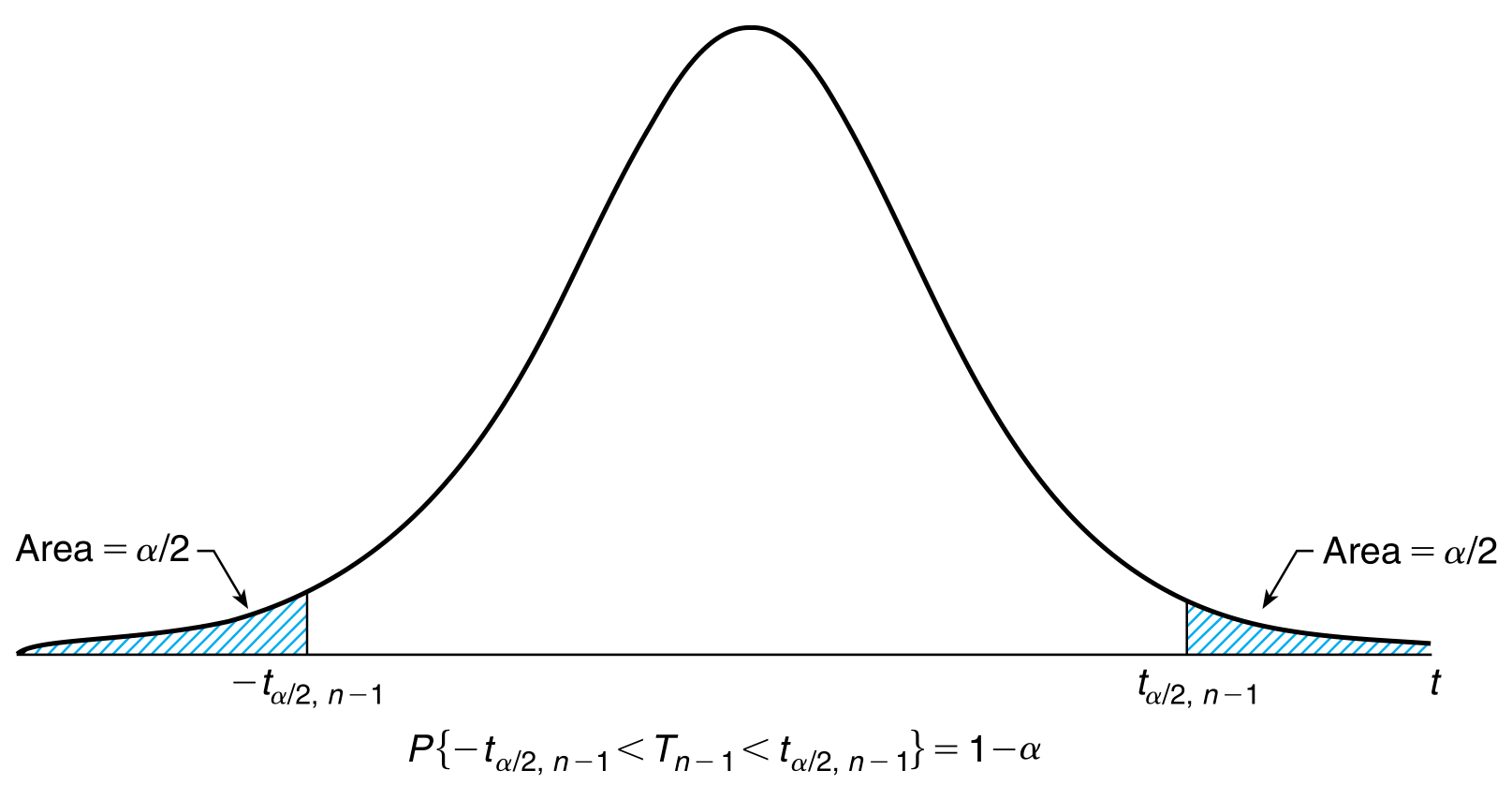
The derivation of confidence intervals in this case is similar to the above, with the only difference of using a t-distribution. Recall \begin{align} \sqrt{n} \frac{\overline{X} - \mu}{S} \sim t_{n-1} \end{align} where $S$ is the sample variance. Following similar derivation to the known variance case, \begin{align} \text{two sided $1 - \alpha$ confidence interval} &= (\overline{x}-t_{\alpha /2, n-1}\frac{s}{\sqrt{n}}, \overline{x}+t_{\alpha /2, n-1}\frac{s}{\sqrt{n}})\newline \text{Lower $1-\alpha$ confidence interval} &= (-\infty, \overline{x} + t_{\alpha, n-1}\frac{s}{\sqrt{n}})\newline \text{Upper $1-\alpha$ confidence interval} &= (\overline{x} - t_{\alpha, n-1}\frac{s}{\sqrt{n}}, \infty) \end{align} where $s$ is the observed value of the sample variance $S$. However, notice that the intervals calculated will usually be larger than those when the variance is known because t-distribution is heavier tailed than a standard normal and thus has higher variance.

Confidence interval for Variance of Normal Distribution when Mean is Unknown

Recall that \begin{align} (n-1)\frac{S^{2}}{\sigma^{2}} \sim \chi_{n-1}^{2} \end{align} By noting that $\sigma^{2}$ is always positive, we have the following \begin{align} \text{two sided $1 - \alpha$ confidence interval} &= (\frac{(n-1)s^{2}}{\chi_{\alpha/2, n-1}^{2}}, \frac{(n-1)s^{2}}{\chi_{1 - \alpha/2, n-1}^{2}})\newline \text{Lower $1-\alpha$ confidence interval} &= (0, \frac{(n-1)s^{2}}{\chi_{1 - \alpha, n-1}^{2}})\newline \text{Upper $1-\alpha$ confidence interval} &= (\frac{(n-1)s^{2}}{\chi_{\alpha, n-1}^{2}}, \infty) \end{align}

Estimating Difference in Means of Two Normal Populations

Suppose the following two independent sets of random variables \begin{align} X_{1}, X_{2}, \ldots, X_{n} &\sim \mathcal{N}(\mu_{1}, \sigma_{1}^{2})\newline Y_{1}, Y_{2}, \ldots, Y_{m} &\sim \mathcal{N}(\mu_{2}, \sigma_{2}^{2}) \end{align}

Then, we are interseted in the distribution of $\mu_{1} - \mu_{2}$. It is intuitive to see that the MLE estimator of this quantity is nothing but $\overline{X} - \overline{Y}$. Also, since $\overline{X}$ and $\overline{Y}$ are both normally distributed, \begin{align} \overline{X} - \overline{Y} \sim \mathcal{N}(\mu_{1} - \mu_{2}, \frac{\sigma_{1}^{2}}{n} + \frac{\sigma_{2}^{2}}{m}) \end{align}

Consequently, using the confidence intervals derived for the case of a mean of a single normal distribution, we have the following intervals when the standard deviations are known \begin{align} \text{two sided $1 - \alpha$ confidence interval} &= (\overline{x} - \overline{y}-z_{\alpha /2}\sqrt{\frac{\sigma_{1}^{2}}{n} + \frac{\sigma_{2}^{2}}{m}}, \overline{x} - \overline{y}+z_{\alpha /2}\sqrt{\frac{\sigma_{1}^{2}}{n} + \frac{\sigma_{2}^{2}}{m}})\newline \text{Lower $1-\alpha$ confidence interval} &= (-\infty, \overline{x} - \overline{y}+z_{\alpha /2}\sqrt{\frac{\sigma_{1}^{2}}{n} + \frac{\sigma_{2}^{2}}{m}})\newline \text{Upper $1-\alpha$ confidence interval} &= (\overline{x} - \overline{y}-z_{\alpha /2}\sqrt{\frac{\sigma_{1}^{2}}{n} + \frac{\sigma_{2}^{2}}{m}}, \infty) \end{align} where $\overline{x}$ and $\overline{y}$ are estimates of $\overline{X}$ and $\overline{Y}$ respectively.

A more challenging scenario arises when the variances are not known. In that case, it is only logical to try to estimate the intervals using sample variances (themselves random variables) \begin{align} S_{1}^{2} &= \frac{\sum_{i=1}^{n} (X_{i} - \overline{X})^{2}}{n-1}\newline S_{2}^{2} &= \frac{\sum_{i=1}^{m} (Y_{i} - \overline{Y})^{2}}{m-1} \end{align}

However, the distribution useful for deriving the confidence intervals \begin{align} \frac{\overline{X} - \overline{Y} - (\mu_{1} - \mu_{2})}{\sqrt{\frac{S_{1}^{2}}{n} + \frac{S_{2}^{2}}{m}}} \end{align} is complicated and depends on the unknown variances. The variable is friendly if we assume that the two unknown variances are both same.

Assuming $\sigma_{1} = \sigma_{2} = \sigma$, it follows \begin{align} (n-1)\frac{S_{1}^{2}}{\sigma^{2}} &\sim \chi_{n-1}^{2}\newline (m-1)\frac{S_{2}^{2}}{\sigma^{2}} &\sim \chi_{m-1}^{2}\newline (n-1)\frac{S_{1}^{2}}{\sigma^{2}} + (m-1)\frac{S_{2}^{2}}{\sigma^{2}} &\sim \chi_{n+m-2}^{2}\newline \end{align} since $S_{1}^{2}$ and $S_{2}^{2}$ are independent chi-square random variables and from section that the sum of such variables is also chi-square.

We already know \begin{align} \frac{\overline{X} - \overline{Y} - (\mu_{1} - \mu_{2})}{\sqrt{\frac{\sigma^{2}}{n} + \frac{\sigma^{2}}{m}}} \sim \mathcal{N}(0, 1) \end{align} and we also know that the ratio of a standard normal and the square root of a chi-square divided by it’s degrees of freedom is a t-distribution \begin{align} \frac{\overline{X} - \overline{Y} - (\mu_{1} - \mu_{2})}{\sqrt{\frac{\sigma^{2}}{n} + \frac{\sigma^{2}}{m}}} \div \sqrt{\frac{(n-1)\frac{S_{1}^{2}}{\sigma^{2}} + (m-1)\frac{S_{2}^{2}}{\sigma^{2}}}{n+m-2}} &\sim t_{n+m-2} \end{align} Let \begin{align} S_{p}^{2} &= \frac{(n-1)S_{1}^{2} + (m-1)S_{2}^{2}}{n + m - 2} \end{align} Then, \begin{align} P(-t_{\alpha/2, n+m-2} \leq \frac{\overline{X} - \overline{Y} - (\mu_{1} - \mu_{2})}{S_{p}\sqrt{\frac{1}{n} + \frac{1}{m}}} \leq t_{\alpha/2, n+m-2}) &= 1 - \alpha \end{align} \begin{align} \text{Two sided $1 - \alpha$ confidence interval} &= (\overline{x} - \overline{y}-t_{\alpha /2, n+m-2}s_{p}\sqrt{\frac{1}{n} + \frac{1}{m}}, \overline{x} - \overline{y}+t_{\alpha /2, n+m-2}s_{p}\sqrt{\frac{1}{n} + \frac{1}{m}}) \end{align} where $s_{p}$ is the sample estimate for $S_{p}$. Lower confidence interval is derived in a similar fashion to the previous derivations, but the upper confidence interval is the lower confidence interval of $\mu_{2} - \mu_{1}$.

Confidence Interval for Mean of Bernoulli Random Variable

Suppose we obtain a sample of $n$ independent Bernoulli random variables, where the probability of success is $p$. Let $X$ denote the no of successes. Using the CLT for large $n$, \begin{align} \frac{X - np}{\sqrt{np(1-p)}} \sim \mathcal{N}(0, 1) \end{align} It is not tractable to calculate the confidence intervals from this formulation. Let $\hat{p} = X/n$ denote the MLE of the mean $p$. Substituiting in the denominator of above, \begin{align} P(-z_{\alpha/2} \leq \frac{X - np}{\sqrt{n\hat{p}(1-\hat{p})}} \leq z_{\alpha/2}) &\approx 1-\alpha\newline \text{Two sided $1-\alpha$ confidence interval} &\approx (\hat{p} - z_{\alpha/2}\sqrt{\frac{\hat{p}(1-\hat{p})}{n}}, \hat{p} + z_{\alpha/2}\sqrt{\frac{\hat{p}(1-\hat{p})}{n}}) \end{align} and one sided confidence intervals can be obtained in similar manner to previous derivations.

Difference of two Populations

The above idea can be extended for interval estimate of the difference of two population ratios. Suppose $X_{1}$ and $X_{2}$ denote the two populations with the proportion estimates $\hat{p_{1}}$ and $\hat{p_{2}}$. Then we have

\begin{align} \bar{X_{1}} - \bar{X_{2}} &\sim \mathcal{N}\roundbr{\hat{p_{1}} - \hat{p_{2}}, \sigma_{d}^{2}}\newline \text{where} \quad \sigma_{d}^{2} &\sim \frac{\hat{p_{1}}(1 - \hat{p_{1}})}{n_{1}} + \frac{\hat{p_{2}}(1 - \hat{p_{2}})}{n_{2}} \end{align}

by the CLT. The $(1-\alpha)100%$ confidence interval becomes \begin{align} \hat{p_{1}} - \hat{p_{2}} \pm z_{\alpha/2}\sigma_{d}^{2} \end{align}