Walkthrough Example
In this section, we look at fitting a SARIMA model on the USAccDeaths data set which contains the number of total accidental deaths in USA at a monthly levels. The data set has two columns, the year-month column and the deaths total. Complete code is avaialable in file time_series_python.py
- We begin by plotting the data.
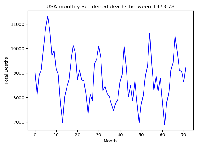
- We notice that there is a seasonality component involved. Also, the mean of the series is not 0. Let’s start by doing a seasonal difference first.
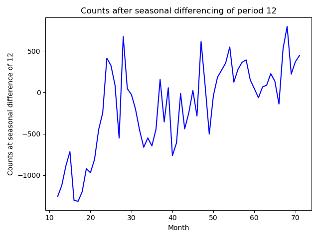
- There is still some trend. A simple $1^{st}$ order difference should remove this trend.
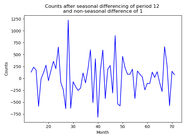
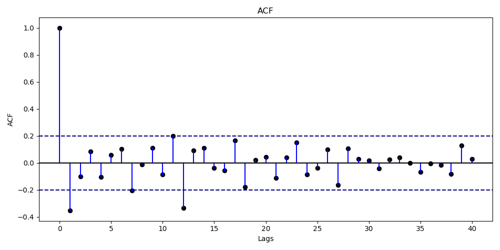
- This is an almost stationary series. We continue the analysis by preparing the ACF and PACF.
-
From the ACF plot, there are only two peaks that are separated by a lag of 12. Hence, the non-seasonal MA is $\leq 1$ and seasonal MA $\leq 1$.
-
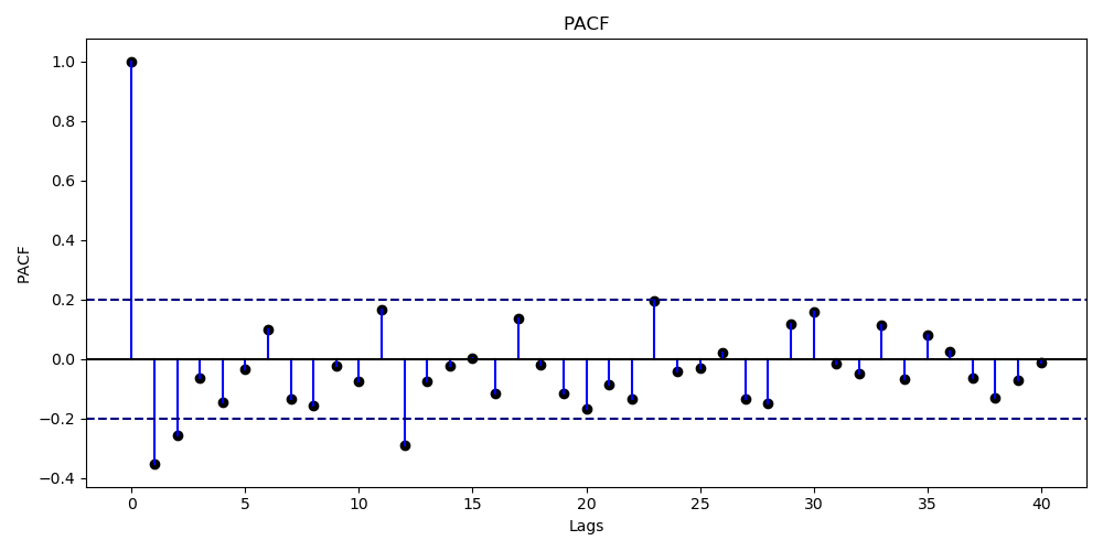
From the PACF plot, there are two nearby peaks at lag 1 and 2, and there is one more peak at lag 12. Hence, the non-seasonal AR is $\leq 2$ and seasonal AR $\leq 1$.
-
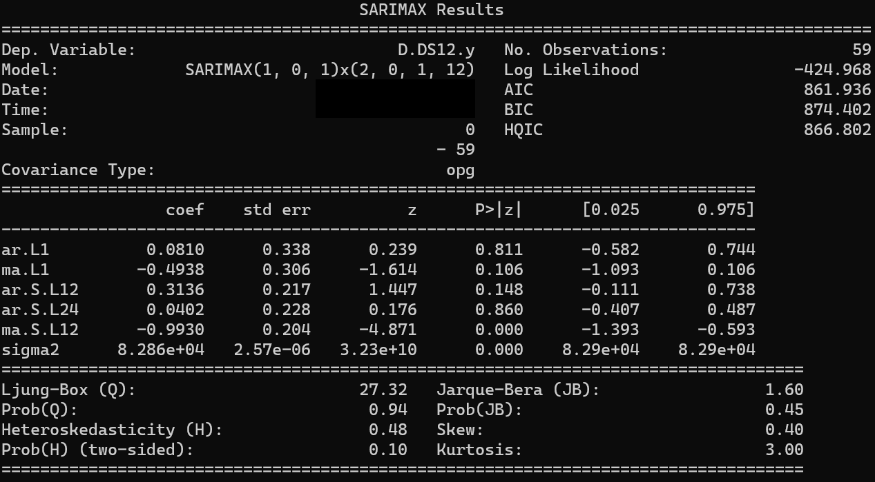
We chose the model $(p,d,q,P,D,Q) = (0,1,1,0,1,1)$ after checking the AIC for various combinations and following the rule of thumb that $p+d+q+P+D+Q \leq 6$..
-
Our model equation becomes \begin{align} (1-B)(1-B^{12})X_{t} &= (1 - 0.4303B)(1 - 0.5527B^{12})Z_{t}\newline Z_{t} &\sim \mathcal{N}(0, 99350) \end{align} and model summary is shown in previous figure.
-
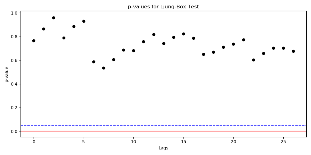
We check the QQ plot to confirm that the residuals are indeed normally distributed. We also check for any correlations between the residuals.
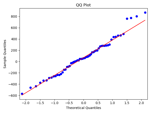
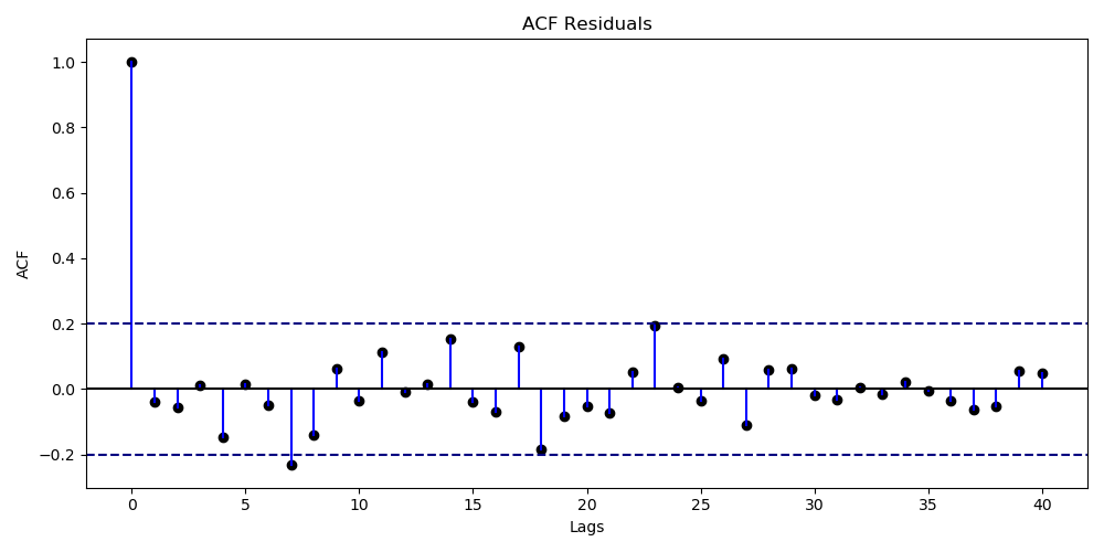
- Barring the noise, no such significant correlations exist. Ljung Box text on the residuals further confirms this. (High $p-values$ imply that we can accept the null hypothesis which is that the data points are independent)