Support Vector Classifier

The previous section was the best case scenario when all observations are perfectly separable. But in real data, this is seldom the case and we encounter the scenario that some observations will be misclassified. To take this into account, we maintain the same optimization as the previous section, but introduce new slack variables to account for the misclassified points \begin{align} &\maximize_{\beta_{0},\ldots,\beta_{p}, M} M\newline &\text{subject to} \quad \sum_{i=1}^{p} \beta_{i}^{2} = 1,\newline &\text{and} \quad y_{i}(\beta_{0} + \beta_{1}x_{i1} + \cdots + \beta_{p}x_{ip}) \geq M(1-\epsilon_{i}) \quad \forall \quad i = 1, 2, \ldots, n\newline &\epsilon_{i} > 0, \sum_{i=1}^{n}\epsilon_{i} \leq C \end{align}

which simply means that if

1. $\epsilon_{i} = 0$, we have correctly classified the observation

2. $\epsilon_{i} < 1$, the observation is correctly classified, but lies between the hyperplane and the margin, thus violating the margin

3. $\epsilon_{i} > 1$, the observation is misclassified

The term $C$ is tells how much of the margin we have violated. Observations on the correct side of the margin will have no contribution to this value. Only the ones violating the margin or the hyperplane will contribute.

Another thing to notice is the use of $M(1-\epsilon)$ in the inequality instead of simply$M - \epsilon$. The first term denots the relative difference in margin while the second term gives the actual difference. Both the formulations lead to different solutions as the former is convex optimization and the latter is non convec. Further, using the former, we can formulate the problem in a manner similar to the maximum margin classifier

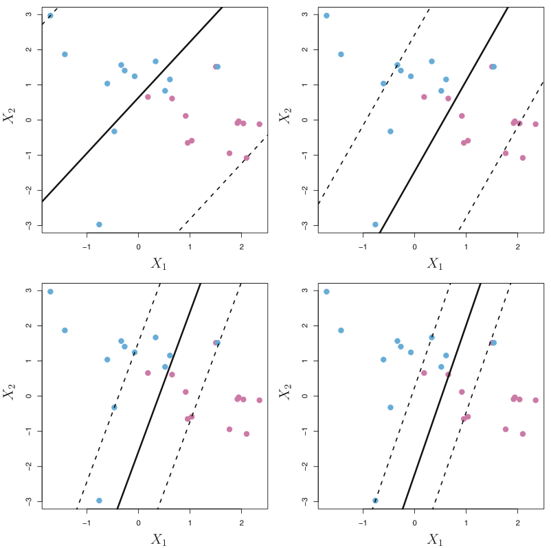
\begin{align} &\minimize_{\beta_{0}, \beta} \frac{1}{2}\lVert \beta \rVert^{2} + C\sum_{j=1}^{N}\epsilon_{j}\newline &\text{subject to} \quad (1-\epsilon_{j}) - y_{i}(\beta_{0} + \beta^{T}x_{i}) \leq 0, : -\epsilon \leq 0 \quad \forall \quad i = 1, 2, \ldots, N\newline \end{align} Replacing the constraint on the sum of the slack variables with a simple $C * sum$ is similar to one done in ridge or lasso shrinkages (section [sec:alternative_ridge_lasso]{reference-type=”ref” reference=”sec:alternative_ridge_lasso”}). $C$ is a constant and will limit how much error we are wiling to tolerate. $C = \inf$ gives us the original separable case since that forces all the $\epsilon$ to be $0$. As we decrease $C$, the epsilons are allowed to take larger values we are allowing more points to be misclassified leading to narrower margins (in figure below).

The Lagrangian becomes \begin{align} L = \frac{1}{2}\lVert \beta \rVert^{2} + C\sum_{j=1}^{N}\epsilon_{j} + \sum_{j=1}^{N} \lambda_{j}((1-\epsilon_{j}) - y_{i}(\beta_{0} + \beta^{T}x_{i})) + \sum_{j=1}^{N} \mu_{j}(-\epsilon_{j}) \end{align} where $\lambda = (\lambda_{1}, \ldots, \lambda_{N})^{T}$, $\mu = (\mu_{1}, \ldots, \mu_{N})^{T}$ and $\epsilon = (\epsilon_{1}, \ldots, \epsilon_{N})^{T}$ and the Wolfe Dual is (all functions in $L$ are differentiable) \begin{align} \max_{\beta_{0}, \beta, \epsilon} L\newline \text{subject to} \quad \lambda > 0, \; \mu>0, \; \frac{\partial L}{\partial \beta} = 0, \; \frac{\partial L}{\partial \beta_{0}} = 0, \; \frac{\partial L}{\partial \epsilon_{j}} = 0 \end{align}

The derivatives equations give the following results \begin{align} \frac{\partial L}{\partial \beta} = 0 \; \implies \beta - \sum_{j=1}^{N}\lambda_{j}y_{j}x_{j} = 0\newline \frac{\partial L}{\partial \beta_{0}} = 0 \; \implies \sum_{j=1}^{N} \lambda_{j}y_{j} = 0\newline \frac{\partial L}{\partial \epsilon_{j}} = 0 \; \implies C - \lambda_{j} - \mu_{j} = 0 \end{align}

Substituiting in the dual leaves us with only $\lambda$ as the variable \begin{align} L &= \frac{1}{2}\beta^{T}\beta + C\sum_{j=1}^{N}\epsilon_{j} + \sum_{j=1}^{N}\lambda_{j}(1 - \epsilon_{j}) - \beta^{T}(\sum_{j=1}^{N} \lambda_{j}y_{j}x_{j}) - \beta_{0}\sum_{j=1}^{N}\lambda_{j}y_{j} - \sum_{j=1}^{N}(C - \lambda_{j})\epsilon_{j}\newline &= \frac{1}{2}\beta^{T}\beta + \sum_{j=1}^{N}\lambda_{j} -\beta^{T}\beta = -\frac{1}{2}\beta^{T}\beta + \sum_{j=1}^{N}\lambda_{j}\newline &= \sum_{j=1}^{N}\lambda_{j} - \frac{1}{2} \sum_{i=1}^{N}\sum_{j=1}^{N} \lambda_{i}\lambda_{j}y_{i}y_{j}x_{i}^{T}x_{j} \end{align}

which we maximize subject to the constraints \begin{align} 0 \leq \lambda \leq C \quad \text{and} \quad \sum_{j=1}^{N}\lambda_{j}y_{j} = 0 \end{align} where the first inequality stems from the fact that $\mu = C - \lambda \geq 0$. Thus, the formulation is very similar to the maximum margin classifier with some additional constraints that allow relaxation of some misclassifications.

Additionally, the optimal values satisfy the KKT conditions \begin{align} \lambda_{j}^{*}((1 - \epsilon^{*}_{j}) - y_{j}(\beta^{*T}x_{j} + \beta_{0}^{*})) = 0, \quad \mu_{j}^{*}\epsilon_{j}^{*} = 0 \end{align} in addition to the all the original and derived constraints (which any solution must satisfy).

Continuing the analogy from maximum margin classifier, only the points that are on the margin or between the margin will participate in determining the separating hyperplane. All such points are called support vectors, since they are literally supporting the determination of the boundary. For all the others, $\lambda_{j} = 0$ and the inquality $y_{j}(\beta^{T}x_{j} + \beta_{0}) \geq 1$ is exactly satisfied.