Hypothesis Testing

Hypothesis testing is a set of procedures used to test a hypothesis about statistical parameters. Based on the results of the procedure, we decide whether to accept or reject the hypothesis. This can be as simple as deciding whether the mean of a population is more than 1 or not.

Whenever a hypothesis is accepted, it does not mean that the hypothesis is true, but rather that the data is consistent with it.

Suppose we have a population that is characterized by the distribution $F_{\theta}$ and we are interested in making statistical comments about the value of the parameters $\theta$. The hypothesis that specifies the statement that we are going to test about the parameter is called the null hypothesis and is denoted by $H_{0}$. Note that the statement of the null hypothesis can either comment on the exact value of the parameter, or comment on an inequality satisfied by the parameter. When the hypothesis completely specifies the distribution, it is called a simple hypothesis and in the other case, it is called composite hypothesis.

To test the hypothesis, suppose we have available with us $n$ independent samples from the population. Based on these samples, we must define a $n$ dimensional region $C$ such that if the sample falls in this region, we reject the null hypothesis and vice versa. This region $C$ is called the critical region (or the rejection region). \begin{align} \text{Reject}\quad H_{0} \quad\text{if}\quad (X_{1}, X_{2}, \ldots, X_{n}) \in C\newline \text{Acecpt}\quad H_{0} \quad\text{if}\quad (X_{1}, X_{2}, \ldots, X_{n}) \notin C \end{align}

It is also important to distinguish simple hypothesis at this point. A hypothesis like $H_{0}: \theta = \theta_{0}$ completely specifies the underlying distribution and is called a simple hypothesis. While a hypothesis like $H_{0}: \theta < \theta_{0}$ does not specify the underlying distribution completely and is rather composed of multiple simple hypothesis. It is called a composite hypothesis.

Null vs Alternate Hypothesis

Often, we also test two hypothesis against each other, called the null and alternate hypothesis. Suppose, the parameter of interest $\theta \in \Omega$; we test $H_{0}$ that is $\theta \in \omega_{0}$ vs $H_{1}$ which is $\theta \in \omega_{1}$ such that $\omega_{0} \cup \omega_{1} = \Omega$ as the null and alternate hypothesis respectively.

Usually null hypothesis corresponds to no change/no difference from the past in the value of the parameter, while the alternate hypothesis corresponds to no change in difference. It is also called the researcher’s hypothesis.

To relate with the critical region above, accepting $H_{0}$ would correspond to rejecting $H_{1}$ and vice versa.

Note that critical region corresponds to rejecting or accepting the null hypothesis and is based on the region where the sample lies. However, the hypothesis itself specifies the region where the parameters lie ($\omega_{0}$ or $\omega_{1}$). The two should not be mixed. Hence, we reject $H_{0}$ if the sample lies in the critical region, and if $H_{0}$ is true, we use the fact that $\theta \in \omega_{0}$.

Errors

Two types of errors can result when checking a hypothesis

type $I$ error: Reject $H_{0}$ when it is correct
type $II$ error: Accept $H_{0}$ when it is incorrect

Since hypothesis testing is about checking if the given data is consistent with the hypothesis, the error we make on rejecting the hypothesis when it is correct should be low. This is consistent with the confidence intervals discussed earlier. We denote type I error by $\alpha$ meaning that there is only $\alpha$ chance that the hypothesis will be incorrectly rejected by the test, and is called the level of significance of the test.

A lower significance level or lower $\alpha$ implies that we require stronger evidence against the null hypothesis to reject it.

A classical approach while testing the parameters of a population will be to first determine a point estimator of the parameter and then determine the distribution of the said estimator. Hypothesis test will usually involve checking whether the estimator lies in a selcted region, for which we can determine the relevant confidence intervals through the distribution of the estimator.

Often, we consider Type I error to be the worse of the two. We usually select critical regions that bind the probability of Type I error and then among those choose the one that minimizes the probability of Type II error.

Size of the Test

The maximum probability of type $I$ error is also called the size of the test. For a simple hypothesis test \begin{align} \alpha &= P(\text{Reject}\; H_{0}\; \text{when it is correct})\newline &= P((X_{1}, X_{2}, \ldots, X_{n}) \in C \vert H_{0})\newline \end{align}

If we write in terms of the regions $\Omega$ \begin{align} \alpha &= sup_{\theta \in \omega_{0}} P(\text{Reject}\; H_{0})\newline &= sup_{\theta \in \omega_{0}} P((X_{1}, X_{2}, \ldots, X_{n}) \in C) \end{align} where $\theta \in \omega_{0}$ corresponds to the region where $H_{0}$ is true.

Finally, the power of a test and any related measure will be defined based on the set of observables $(X_{1}, X_{2}, \ldots, X_{n})$ since the hypothesis tests depend on determining the critical region $C$ for these set of observables.

With composite hypothesis, $\alpha$ will be called the maximum probability of comitting a Type I error.

Power of a Test

Over all critical regions of size $\alpha$, we want to minimize the probability of Type II error. We consider a slightly different metric for this \begin{align} 1 - P_{\theta}(\text{Type II error}) &= P(\text{Reject $H_{0}$}\vert text{$H_{0}$ is false})\newline &= P((X_{1}, X_{2}, \ldots, X_{n}) \in C) \end{align}

Since we are rejecting $H_{0}$, the alternate must be true and $\theta \in \omega_{1}$. Further, as our intent was to minimize the Type II error, we can equivalently maximize the power defined above. The power function is defined as \begin{align} \gamma_{C}(\theta) = P_{\theta}((X_{1}, X_{2}, \ldots, X_{n}) \in C) \quad \theta \in \omega_{1} \end{align} For two critical regions with the same size $\alpha$, we consider the one with higher power (or lower Type II error) to be the better one.

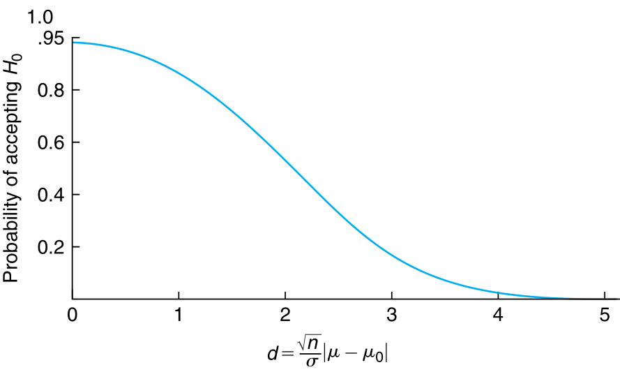
Usually the power function is monotonic and decreasing for a fixed $\alpha$ as shown below (and discussed later)

Curve of $\beta(\mu)$ for a fixed $\alpha$

Often, loosely speaking, some may refer to the power function as \begin{align} \gamma_{C}(\theta) = P_{\theta}((X_{1}, X_{2}, \ldots, X_{n}) \in C) \quad \theta \in \Omega \end{align} which is only concerned with the definition of the power function from the perspective of the critical region.