Test around Mean of Normal Population

Known Variance

Consider $n$ samples $X_{1}, X_{2}, \ldots, X_{n}$ drawn from a normal distribution with unknown mean $\mu$ and known variance $\sigma^{2}$. We have the following hypothesis \begin{align} \text{null hypothesis} \quad H_{0}&: \mu = \mu_{0}\newline \text{alternate hypothesis} \quad H_{1}&: \mu \neq \mu_{0} \end{align}

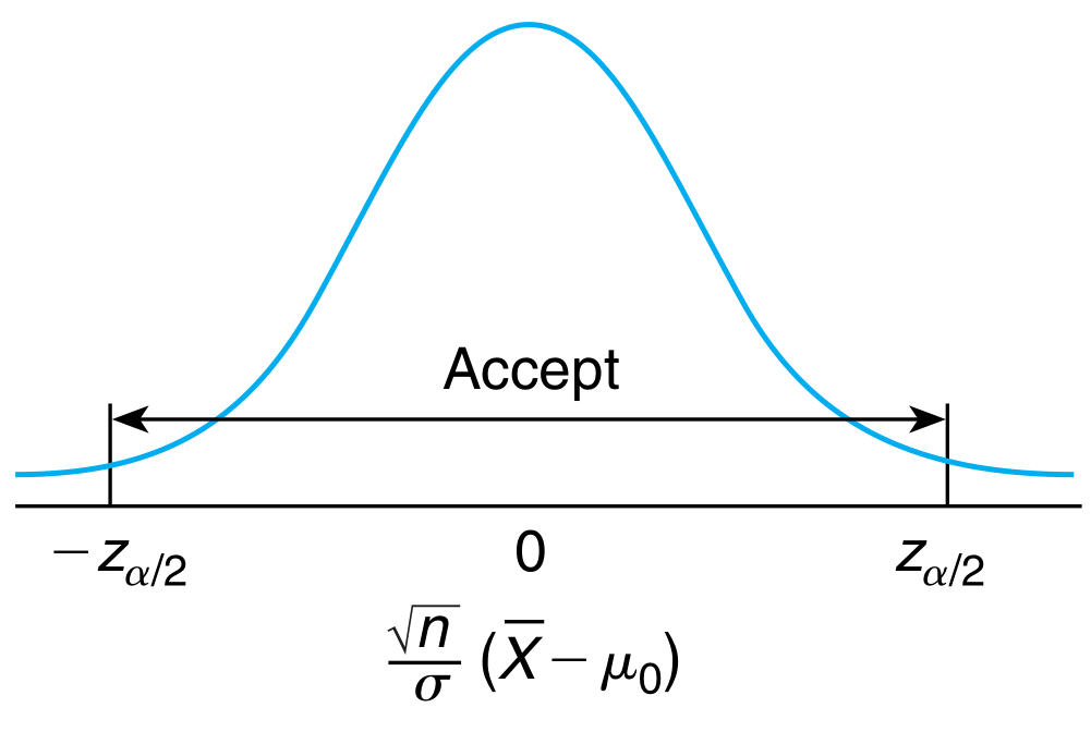
The sample mean $\overline{X}$ is clearly a natural choice for the estimator of the mean. It is intuitive to define the critical region in such a manner that we reject $H_{0}$ if the estimator is far off from $\mu_{0}$ and vice versa \begin{align} C = { X_{1}, X_{2}, \ldots X_{n}: \vert\overline{X} - \mu_{0}\vert > c} \end{align} for some suitably chosen $c$. We also know that the mean of a normal population has a normal distribution. Hence for some significance level $\alpha$ (type I error), \begin{align} P_{\mu_{0}}(\vert\overline{X} - \mu_{0}\vert > c) = \alpha \end{align} where the subscript denotes the fact that the probability is being calculated under the assumption of $\mu = \mu_{0}$. Under this assumption, $\overline{X}$ is normally distributed with mean $\mu_{0}$. \begin{align} P_{\mu_{0}}(\vert\frac{\overline{X} - \mu_{0}}{\sigma/\sqrt{n}}\vert > \frac{c\sqrt{n}}{\sigma}) &= \alpha\newline 2P_{\mu_{0}}(\frac{\overline{X} - \mu_{0}}{\sigma/\sqrt{n}} > \frac{c\sqrt{n}}{\sigma}) &= \alpha \end{align} but we know that these are tabulated values \begin{align} P(Z > z_{\alpha/2}) &= \alpha/2\newline \text{or,}\quad \frac{c\sqrt{n}}{\sigma} &= z_{\alpha/2}\newline \text{or,}\quad c &= \frac{\sigma z_{\alpha/2}}{\sqrt{n}} \end{align} or simply put in terms of the hypothesis test, \begin{alignat}{4} \text{Reject}\quad &H_{0} \quad\text{if}\quad &\bigg\lvert \frac{\sqrt{n}}{\sigma}(\overline{X} - \mu_{0}) \big\rvert &> &z_{\alpha/2}\newline \text{Accept}\quad &H_{0} \quad\text{if}\quad &\big\lvert \frac{\sqrt{n}}{\sigma}(\overline{X} - \mu_{0}) \big\rvert &\leq &z_{\alpha/2}\newline \end{alignat} where $\alpha$ is the type I error and should ideally be low.

Acceptance Region for Hypothesis $\mu=\mu_{0}$

p-value

p-value denotes the probability of observing a test-statistic at least as large as the observed test-statistic under the assumption that the null hypothesis is true. Mathemtically, \begin{align} P(Z > \frac{\sqrt{n}}{\sigma}(\overline{X} - \mu_{0})) = \text{p-value} \end{align} where $Z$ is the random variable denoting the test-statistic while right-hand side of the inequality is the observed test-statistic. For the above formula, we have assumed the test statistic to be derived from a normal distribution. However, the definition is applicable to any distribution.

A very small p-value means that either the null hypothesis is incorrect, or the observed test statistic must be very unlikely. We can use p-value to compare against already defined significance levels to accept or reject the null hypothesis.

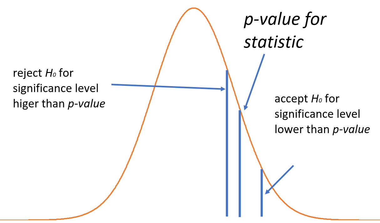
*p-value* and significance levels on a standard normal distribution

Furthermore, if we have a predefined value of the significance level, any p-value lower than this level implies it is very likely for the mean to be different, calling for rejecting $H_{0}$. This is visually represented in figure above (note that the figure compares different significance levels for a fixed value of p-value).

Thus, a small p-value denotes strong evidence in favor of observing an effect. For an analogy, consider the hypothesis test concerning the weights of a linear regression model. The usual $H_{0}$ refers to the coefficient being $0$. Thus, a small p-value strongly rejects the null hypothesis, meaning that the corresponding regressor has non-zero impact on the target variable.

Power of a test and Type II error

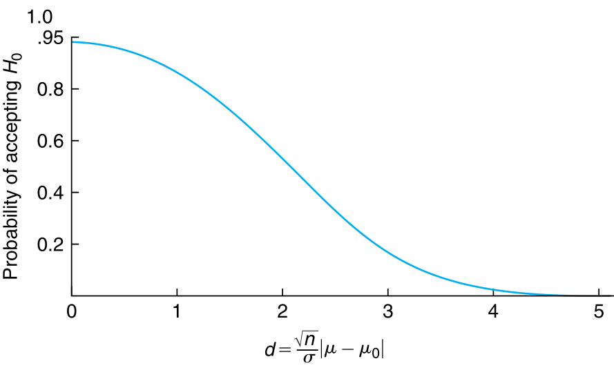
We have not yet invoked the type II error. Consider $\beta(\mu)$ as probability of accepting $H_{0}$ when the mean is $\mu$ \begin{align} \beta(\mu) &= P_{\mu}(\text{accepting $H_{0}$ when the mean is $\mu$})\newline &= P(\text{statistic is}\quad \leq z_{\alpha/2})\newline &= P(\vert\frac{\sqrt{n}}{\sigma}(\overline{X} - \mu_{0})\vert \leq z_{\alpha/2})\newline &= P(-z_{\alpha/2} \leq \frac{\sqrt{n}}{\sigma}(\overline{X} - \mu_{0}) \leq z_{\alpha/2}) \end{align} We also define effect size here. It is defined as \begin{align} \text{effect size} &= \text{True value} - \text{Hypothesize value}\newline &= \mu - \mu_{0} \end{align} But, under the premise that $\mu$ is the correct mean (and $H_{0}$ is false), \begin{align} \frac{\overline{X} - \mu}{\sigma/\sqrt{n}} \sim \mathcal{N}(0, 1) \end{align} Thus, \begin{align} \beta(\mu) &= P(-z_{\alpha/2} - \frac{\sqrt{n}}{\sigma}\mu \leq \frac{\sqrt{n}}{\sigma}(\overline{X} - \mu_{0}) - \frac{\sqrt{n}}{\sigma}\mu \leq z_{\alpha/2} - \frac{\sqrt{n}}{\sigma}\mu)\newline &= P(-z_{\alpha/2} - \frac{\sqrt{n}}{\sigma}(\mu + \mu_{0}) \leq \frac{\sqrt{n}}{\sigma}(\overline{X} - \mu) \leq z_{\alpha/2} - \frac{\sqrt{n}}{\sigma}(\mu + \mu_{0}))\newline &= \Phi(z_{\alpha/2} - \frac{\sqrt{n}}{\sigma}(\mu - \mu_{0})) - \Phi(-z_{\alpha/2} - \frac{\sqrt{n}}{\sigma}(\mu - \mu_{0}))\newline &= \Phi(\frac{\sqrt{n}}{\sigma}(\mu_{0} - \mu) +z_{\alpha/2}) - \Phi(\frac{\sqrt{n}}{\sigma}(\mu_{0} - \mu) -z_{\alpha/2})\newline \end{align} where $\Phi$ is the standard normal cumulative distribution function.

$\beta(\mu)$ is called the Operating Charectistic. The value of this function is only dependent on the gap between $\mu_{0}$ and $\mu$. For a fix $\alpha$, as the gap grows, we move away from the centre of the standard normal. As such, the difference in the two terms of $\beta(\mu)$ keeps decreasing. It is maximum when $\mu = \mu_{0}$.

Curve of $\beta(\mu)$ for a fixed $\alpha$

The function $1 - \beta(\mu)$ is called the power function and is the probability of rejection of $H_{0}$ when it is false. This function is useful in calculating the value of the sample size so that the probability of accepting $H_{0}: \mu = \mu_{0}$ when the true mean is $\mu_{1}$ is $\beta$. We solve the equation $\beta(\mu_{1}) = \beta$ and try to guess the value of $n$ because analytical solution is not possible.

\begin{align} n \approx \frac{(z_{\alpha/2} + z_{\beta})^{2} \sigma^{2}}{(\mu_{1} - \mu_{0})^{2}} \end{align} is the approximate solution assuming $\alpha$ is negligible.

The power of a test is dependent on

Sample size $n$: Other things being constant, the power of a test is higher the larger the sample size.
Significance level $\alpha$: The smaller the value of $\alpha$, the larger is the acceptance region making it more likely to accept $H_{0} (\mu = \mu_{0})$ when the true mean is different.
Effect size: The greater the effect size (difference between the hypothesized value and the true value), the higher the power of the test.

Neyman-Pearson Lemma

Consider a test with two competing hypothesis $H_{0} = \theta_{0}$ and $H_{1} = \theta_{1}$ where the probability density (or mass) function is given by $f(\mathbf{x} \vert \theta_{i})$ for $i \in {0, 1}$. Denoting the critical region (rejection region) by $C$, the Neyman-Pearson Lemma states that the Most Powerful (MP) test statisfies the below for some $\eta \geq 0$

$\mathbf{x} \in C \; \text{if} \; f(\mathbf{x}\vert\theta_{1}) > \eta f(\mathbf{x}\vert\theta_{0})$
$\mathbf{x} \in C^{c} \; \text{if} \; f(\mathbf{x}\vert\theta_{1}) < \eta f(\mathbf{x}\vert\theta_{0})$
$P_{\theta_{0}}(\mathbf{X} \in C) = \alpha$ for some prefixed significance level $\alpha$

In practice, the likelihood ratio is often used to construct the tests and determine the relation between the effect size and the likelihood ratio.

One Sided Test

In one sided test, we test the equality of the mean with a fixed value vs a single sided inequality of the mean being larger than, or smaller than that fixed value. \begin{align} \text{null hypothesis}\quad H_{0}&: \mu = \mu_{0}\newline \text{alternate hypothesis}\quad H_{1}&: \mu > \mu_{0} \end{align}

Note that the variance of the distribution is known in this case. Clearly, the critical region (rejection region) is one where the large values of $\mu$ are unlikely \begin{align} C = {X_{1}, \ldots, X_{n}: \overline{X} - \mu_{0} > c} \end{align} for some constant $c$ chosen based on the significance level $\alpha$. Equivalently, \begin{align} P(\frac{\overline{X} - \mu_{0}}{\sigma/\sqrt{n}} > z_{\alpha}) &= \alpha\newline \text{or,}\quad \overline{X} &> z_{\alpha}\frac{\sigma}{\sqrt{n}} + \mu_{0} \end{align}

is the rejection region based on the sample mean.

\begin{alignat}{4} \text{Reject}\quad &H_{0} \quad\text{if}\quad &\frac{\sqrt{n}}{\sigma}(\overline{X} - \mu_{0}) &> &z_{\alpha}\newline \text{Accept}\quad &H_{0} \quad\text{if}\quad &\frac{\sqrt{n}}{\sigma}(\overline{X} - \mu_{0}) &\leq &z_{\alpha}\newline \end{alignat}

The p-value is similarly calculated as the probability that the standard normal is at least as large as this test statistic. Similar to the two sided test, operating characteristic curve can be defined \begin{align} \beta(\mu) &= P(\text{Accepting}\quad H_{0})\newline &= P(\overline{X} \leq z_{\alpha}\frac{\sigma}{\sqrt{n}} + \mu_{0})\newline &= P(\frac{\overline{X} - \mu}{\sigma/\sqrt{n}} \leq z_{\alpha} + \frac{\mu_{0} - \mu}{\sigma/\sqrt{n}})\newline &= P(Z \leq z_{\alpha} + \frac{\mu_{0} - \mu}{\sigma/\sqrt{n}}) \end{align} where $Z$ is the standard normal.

Special Note

The tests discussed above have been derived under the assumption that the sample mean has a normal distribution. But, by central limit theorem, the sample mean of any large population will tend towards a normal distribution. Hence, the hypothesis tests will remain valid provided the population has known variance $\sigma^{2}$.

Unknown Variance

We proceed in a manner similar to the known variance case but use sample variance instead. Recall \begin{align} \sqrt{n} \frac{\overline{X} - \mu_{0}}{S} \sim T_{n-1} \end{align} which is a t-distributed random variable with $n-1$ degrees of freedom. Since t-distribution also has specially defined values $t_{\alpha, n-1}$ similar to $z_{\alpha}$, we can simply use the following 2-sided tests at significance level $\alpha$ \begin{alignat}{4} \text{Reject}\quad &H_{0} \quad\text{if}\quad &\bigg \lvert\frac{\sqrt{n}}{S}(\overline{X} - \mu_{0}) \bigg\rvert &> &t_{\alpha/2, n-1}\newline \text{Accept}\quad &H_{0} \quad\text{if}\quad &\bigg \lvert\frac{\sqrt{n}}{S}(\overline{X} - \mu_{0}) \bigg\rvert &\leq &t_{\alpha/2, n-1}\newline \end{alignat}

Further, p-values are defined using the same statistic $\sqrt{n}(\overline{X} - \mu_{0})/S$ and for any significance level which is less than the p-value probability that the t-statistic is greater than this statistic $\sqrt{n}(\overline{X} - \mu_{0})/S$, we will reject $H_{0}: \mu = \mu_{0}$. We accept the null hypothesis when the significance level is larger than the p-value.

Similar to the known variance case, we have the one sided tests defined as below \begin{align} H_{0}: \mu \leq \mu_{0} \quad \text{versus} \quad H_{1}: \mu > \mu_{0} \end{align} \begin{alignat}{4} \text{Reject}\quad &H_{0} \quad\text{if}\quad &\frac{\sqrt{n}}{S}(\overline{X} - \mu_{0}) &> &t_{\alpha, n-1}\newline \text{Accept}\quad &H_{0} \quad\text{if}\quad &\frac{\sqrt{n}}{S}(\overline{X} - \mu_{0}) &\leq &t_{\alpha, n-1}\newline \end{alignat} and the other side \begin{align} H_{0}: \mu \geq \mu_{0} \quad \text{versus} \quad H_{1}: \mu < \mu_{0} \end{align} \begin{alignat}{4} \text{Reject}\quad &H_{0} \quad\text{if}\quad &\frac{\sqrt{n}}{S}(\overline{X} - \mu_{0}) &< &-t_{\alpha, n-1}\newline \text{Accept}\quad &H_{0} \quad\text{if}\quad &\frac{\sqrt{n}}{S}(\overline{X} - \mu_{0}) &\geq &-t_{\alpha, n-1}\newline \end{alignat} and we can calculate the p-value as well in the above cases using the test statistic.